Tag Archives: hockey stick

Phil Jones Interview

I am a bit late on this (I have family over for the weekend) but on the off chance you have not seen it, make sure to check out the notes from the interview of Phil Jones of the CRU.  Here is the BBC Q&A.    Anthony Watt has as good a summary as anyone.

Anthony summarizes as follows:

Specifically, the Q-and-As confirm what many skeptics have long suspected:

  • Neither the rate nor magnitude of recent warming is exceptional.
  • There was no significant warming from 1998-2009. According to the IPCC we should have seen a global temperature increase of at least 0.2°C per decade.
  • The IPCC models may have overestimated the climate sensitivity for greenhouse gases, underestimated natural variability, or both.
  • This also suggests that there is a systematic upward bias in the impacts estimates based on these models just from this factor alone.
  • The logic behind attribution of current warming to well-mixed man-made greenhouse gases is faulty.
  • The science is not settled, however unsettling that might be.
  • There is a tendency in the IPCC reports to leave out inconvenient findings, especially in the part(s) most likely to be read by policy makers.

I think some of these conclusions are a bit of a reach from the Q&A. I don’t get the sense that Jones is abandoning the basic hypothesis that climate sensitivity to manmade CO2 is high (e.g. 3+ degrees per doubling, rather than <=1 degrees as many skeptics would hypothesize).  In particular, I think the writing has been on the wall for a while that alarmists were bailing on the hockey stick / MWP-related arguments as indicative of high sensitivities.

The new news for me was the admission that the warming rate from 1979-present is in no way unprecedented.  This is important as the lead argument (beyond black box “the models say so” justifications) for blaming anthropogenic factors for recent warming is that the rate of warming was somehow unprecedented.  However, Jones admits (as all rational skeptics have said for some time) that the warming rate from 1979 to today is really no different than we have measured in other periods decidedly unaffected by CO2.

I have made this argument before here, with the following chart:

slide48

Again, from Anthony:

Period Length Trend
(Degrees C per decade)
Significance
1860-1880 21 0.163 Yes
1910-1940 31 0.15 Yes
1975-1998 24 0.166 Yes
1975-2009 35 0.161 Yes

Here, by the way, was my attempt to explain the last 100 years of temperature with a cyclical wave plus a small linear trend (my much more transparent and simple climate model)

slide53

Not bad, huh?  Here is a similar analysis using a linear trend plus the PDO

slide54

More Hockey Stick Hyjinx

Update: Keith Briffa responds to the issues discussed below here.

Sorry I am a bit late with the latest hockey stick controversy, but I actually had some work at my real job.

At this point, spending much time on the effort to discredit variations of the hockey stick analysis is a bit like spending time debunking phlogiston as the key element of combustion.  But the media still seems to treat these analyses with respect, so I guess the effort is necessary.

Quick background:  For decades the consensus view was that earth was very warm during the middle ages, got cold around the 17th century, and has been steadily warming since, to a level today probably a bit short of where we were in the Middle Ages.  This was all flipped on its head by Michael Mann, who used tree ring studies to “prove” that the Medieval warm period, despite anecdotal evidence in the historic record (e.g. the name of Greenland) never existed, and that temperatures over the last 1000 years have been remarkably stable, shooting up only in the last 50 years to 1998 which he said was likely the hottest year of the last 1000 years.  This is called the hockey stick analysis, for the shape of the curve.

Since he published the study, a number of folks, most prominently Steve McIntyre, have found flaws in the analysis.  He claimed Mann used statistical techniques that would create a hockey stick from even white noise.  Further, Mann’s methodology took numerous individual “proxies” for temperatures, only a few of which had a hockey stick shape, and averaged them in a way to emphasize the data with the hockey stick.  Further, Mann has been accused of cherry-picking — leaving out proxy studies that don’t support his conclusion.  Another problem emerged as it became clear that recent updates to his proxies were showing declining temperatures, what is called “divergence.”  This did not mean that the world was not warming, but did mean that trees may not be very good thermometers.  Climate scientists like Mann and Keith Briffa scrambled for ways to hide the divergence problem, and even truncated data when necessary.  More hereMann has even flipped the physical relationship between a proxy and temperature upside down to get the result he wanted.

Since then, the climate community has tried to make itself feel better about this analysis by doing it multiple times, including some new proxies and new types of proxies (e.g. sediments vs. tree rings).  But if one looks at the studies, one is struck by the fact that its the same 10 guys over and over, either doing new versions of these studies or reviewing their buddies studies.  Scrutiny from outside of this tiny hockey stick society is not welcome.  Any posts critical of their work are scrubbed from the comment sections of RealClimate.com (in contrast to the rich discussions that occur at McIntyre’s site or even this one) — a site has even been set up independently to archive comments deleted from Real Climate.  This is a constant theme in climate.  Check this policy out — when one side of the scientific debate allows open discussion by all comers, and the other side censors all dissent, which do you trust?

Anyway, all these studies have shared a couple of traits in common:

  • They have statistical methodologies to emphasize the hockey stick
  • They cherry pick data that will support their hypothesis
  • They refuse to archive data or make it available for replication

The some extent, the recent to-do about Briffa and the Yamal data set have all the same elements.  But this one appears to have a new one — not only are the data sets cherry-picked, but there is growing evidence that the data within a data set has been cherry picked.

Yamal is important for the following reason – remember what I said above about just a few data sets driving the whole hockey stick.  These couple of data sets are the crack cocaine to which all these scientists are addicted.  They are the active ingredient.  The various hockey stick studies may vary in their choice of proxy sets, but they all include a core of the same two or three that they know with confidence will drive the result they want, as long as they are careful not to water them down with too many other proxies.

Here is McIntyre’s original post.   For some reason, the data set Briffa uses falls off to ridiculously few samples in recent years (exactly when you would expect more).  Not coincidentally, the hockey stick appears exactly as the number of data points falls towards 10 and then 5 (from 30-40).  If you want a longer, but more layman’s view, Bishop Hill blog has summarized the whole storyUpdateMore here, with lots of the links I didn’t have time this morning to find.

Postscript: When backed against the wall with no response, the Real Climate community’s ultimate response to issues like this is “Well, it doesn’t matter.”  Expect this soon.

Update: Here are the two key charts, as annotated by JoNova:

rcs_chronologies1v2

And it “matters”

yamal-mcintyre-fig2

Data Splices

Splicing data sets is a virtual necessity in climate research.  Let’s think about how I might get a 500,000 year temperature record.  For the first 499,000 years I probably would use a proxy such as ice core data to infer a temperature record.  From 150-1000 years ago I might switch to tree ring data as a proxy.  From 30-150 years ago I probably would use the surface temperature record.  And over the last 30 years I might switch to the satellite temperature measurement record.  That’s four data sets, with three splices.

But there is, obviously, a danger in splices.  It is sometimes hard to ensure that the zero values are calibrated between two records (typically we look at some overlap time period to do this).  One record may have a bias the other does not have.  One record may suppress or cap extreme measurements in some way (example – there is some biological limit to tree ring growth, no matter how warm or cold or wet or dry it is).  We may think one proxy record is linear when in fact it may not be linear, or may be linear over only a narrow range.

We have to be particularly careful at what conclusions we draw around the splices.  In particular, one would expect scientists to be very, very skeptical of inflections or radical changes in the slope or other characteristic of the data that occur right at a splice.  Occam’s Razor might suggest the more logical solution is that such changes are related to incompatibilities with the two data sets being spliced, rather than any particular change in the physical phenomena being measured.

Ah, but not so in climate.  A number of the more famous recent findings in climate have coincided with splices in data sets.  The most famous is in Michael Mann’s hockey stick, where the upward slope at the end of the hockey stick occurs exactly at the point where tree ring proxy data is spliced to instrument temperature measurements.  In fact, if looking only at the tree ring data brought to the present, no hockey stick occurs (in fact the opposite occurs in many data sets he uses).   The obvious conclusion would have been that the tree ring proxy data might be flawed, and that it was not directly comparable with instrumental temperature records.  Instead, Al Gore built a movie around it.  If you are interested, the splice issue with the Mann hockey stick is discussed in detail here.

Another example that I have not spent as much time with is the ocean heat content data, discussed at the end of this post.  Heat content data from the ARGO buoy network is spliced onto older data.  The ARGO network has shown flat to declining heat content every year of its operation, except for a jump in year one from the old data to the new data.  One might come to the conclusion that the two data sets did not have their zero’s matched well, such that the one year jump is a calibration issue in joining the data sets, and not the result of an actual huge increase in ocean heat content of a magnitude that has not been observed before or since.  Instead, headline read that the ARGO network has detected huge increases in ocean heat content!

So this brings us to today’s example, probably the most stark and obvious of the bunch, and we have our friend Michael Mann to thank for that.  Mr. Mann wanted to look at 1000 years of hurricanes, the way he did for temperatures.  He found some proxy for hurricanes in years 100-1000, basically looking at sediment layers.  He uses actual observations for the last 100 years or so as reported by a researcher named Landsea  (one has to adjust hurricane numbers for observation technology bias — we don’t miss any hurricanes nowadays, but hurricanes in 1900 may have gone completely unrecorded depending on their duration and track).  Lots of people argue about these adjustments, but we are not going to get into that today.

Here are his results, with the proxy data in blue and the Landsea adjusted observations in red.  Again you can see the splice of two very different measurement technologies.

mannlandseaunsmoothed

Now, you be the scientist.  To help you analyze the data, Roger Pielke via Anthony Watt has calculated to basic statistics for the blue and red lines:

The Mann et al. historical predictions [blue] range from a minimum of 9 to a maximum of 14 storms in any given year (rounding to nearest integer), with an average of 11.6 storms and a standard deviation of 1.0 storms. The Landsea observational record [red] has a minimum of 4 storms and a maximum of 28 with and average of 11. 7 and a standard deviation of 3.75.

The two series have almost dead-on the same mean but wildly different standard deviations.  So, junior climate scientists, what did you conclude?  Perhaps:

  • The hurricane frequency over the last 1000 years does not appear to have increased appreciably over the last 100, as shown by comparing the two means.  or…
  • We couldn’t conclude much from the data because there is something about our proxy that is suppressing the underlying volatility, making it difficult to draw conclusions

Well, if you came up with either of these, you lose your climate merit badge.  In fact, here is one sample headline:

Atlantic hurricanes have developed more frequently during the last decade than at any point in at least 1,000 years, a new analysis of historical storm activity suggests.

Who would have thought it?  A data set with a standard deviation of 3.75 produces higher maximum values than a data set with the same mean but with the standard deviation suppressed down to 1.0.  Unless, of course, you actually believe that the data volatility in the underlying natural process suddenly increase several times coincidental in the exact same year as the data splice.

As Pielke concluded:

Mann et al.’s bottom-line results say nothing about climate or hurricanes, but what happens when you connect two time series with dramatically different statistical properties. If Michael Mann did not exist, the skeptics would have to invent him.

Postscript #1: By the way, hurricane counts are a horrible way to measure hurricane activity (hurricane landfalls are even worse).  The size and strength and duration of hurricanes are also important.  Researchers attempt to factor these all together into a measure of accumulated cyclone energy.  This metric of world hurricanes and cyclones has actually be falling the last several years.

global_running_ace2

Postscript #2: Just as another note on Michael Mann, he is the guy who made the ridiculously overconfident statement that “there is a 95 to 99% certainty that 1998 was the hottest year in the last one thousand years.”   By the way, Mann now denies he ever made this claim, despite the fact that he was recorded on video doing so.  The movie Global Warming:  Doomsday Called Off has the clip.  It is about 20 seconds into the 2nd of the 5 YouTube videos at the link.

Sudden Acceleration

For several years, there was an absolute spate of lawsuits charging sudden acceleration of a motor vehicle — you probably saw such a story:  Some person claims they hardly touched the accelerator and the car leaped ahead at enormous speed and crashed into the house or the dog or telephone pole or whatever.  Many folks have been skeptical that cars were really subject to such positive feedback effects where small taps on the accelerator led to enormous speeds, particularly when almost all the plaintiffs in these cases turned out to be over 70 years old.  It seemed that a rational society might consider other causes than unexplained positive feedback, but there was too much money on the line to do so.

Many of you know that I consider questions around positive feedback in the climate system to be the key issue in global warming, the one that separates a nuisance from a catastrophe.  Is the Earth’s climate similar to most other complex, long-term stable natural systems in that it is dominated by negative feedback effects that tend to damp perturbations?  Or is the Earth’s climate an exception to most other physical processes, is it in fact dominated by positive feedback effects that, like the sudden acceleration in grandma’s car, apparently rockets the car forward into the house with only the lightest tap of the accelerator?

I don’t really have any new data today on feedback, but I do have a new climate forecast from a leading alarmist that highlights the importance of the feedback question.

Dr. Joseph Romm of Climate Progress wrote the other day that he believes the mean temperature increase in the “consensus view” is around 15F from pre-industrial times to the year 2100.  Mr. Romm is mainly writing, if I read him right, to say that critics are misreading what the consensus forecast is.  Far be it for me to referee among the alarmists (though 15F is substantially higher than the IPCC report “consensus”).  So I will take him at his word that 15F increase with a CO2 concentration of 860ppm is a good mean alarmist forecast for 2100.

I want to deconstruct the implications of this forecast a bit.

For simplicity, we often talk about temperature changes that result from a doubling in Co2 concentrations.  The reason we do it this way is because the relationship between CO2 concentrations and temperature increases is not linear but logarithmic.  Put simply, the temperature change from a CO2 concentration increase from 200 to 300ppm is different (in fact, larger) than the temperature change we might expect from a concentration increase of 600 to 700 ppm.   But the temperature change from 200 to 400 ppm is about the same as the temperature change from 400 to 800 ppm, because each represents a doubling.   This is utterly uncontroversial.

If we take the pre-industrial Co2 level as about 270ppm, the current CO2 level as 385ppm, and the 2100 Co2 level as 860 ppm, this means that we are about 43% through a first doubling of Co2 since pre-industrial times, and by 2100 we will have seen a full doubling (to 540ppm) plus about 60% of the way to a second doubling.  For simplicity, then, we can say Romm expects 1.6 doublings of Co2 by 2100 as compared to pre-industrial times.

So, how much temperature increase should we see with a doubling of CO2?  One might think this to be an incredibly controversial figure at the heart of the whole matter.  But not totally.  We can break the problem of temperature sensitivity to Co2 levels into two pieces – the expected first order impact, ahead of feedbacks, and then the result after second order effects and feedbacks.

What do we mean by first and second order effects?  Well, imagine a golf ball in the bottom of a bowl.  If we tap the ball, the first order effect is that it will head off at a constant velocity in the direction we tapped it.  The second order effects are the gravity and friction and the shape of the bowl, which will cause the ball to reverse directions, roll back through the middle, etc., causing it to oscillate around until it eventually loses speed to friction and settles to rest approximately back in the middle of the bowl where it started.

It turns out the the first order effects of CO2 on world temperatures are relatively uncontroversial.  The IPCC estimated that, before feedbacks, a doubling of CO2 would increase global temperatures by about 1.2C  (2.2F).   Alarmists and skeptics alike generally (but not universally) accept this number or one relatively close to it.

Applied to our increase from 270ppm pre-industrial to 860 ppm in 2100, which we said was about 1.6 doublings, this would imply a first order temperature increase of 3.5F from pre-industrial times to 2100  (actually, it would be a tad more than this, as I am interpolating a logarithmic function linearly, but it has no significant impact on our conclusions, and might increase the 3.5F estimate by a few tenths.)  Again, recognize that this math and this outcome are fairly uncontroversial.

So the question is, how do we get from 3.5F to 15F?  The answer, of course, is the second order effects or feedbacks.  And this, just so we are all clear, IS controversial.

A quick primer on feedback.  We talk of it being a secondary effect, but in fact it is a recursive process, such that there is a secondary, and a tertiary, etc. effects.

Lets imagine that there is a positive feedback that in the secondary effect increases an initial disturbance by 50%.  This means that a force F now becomes F + 50%F.  But the feedback also operates on the additional 50%F, such that the force is F+50%F+50%*50%F…. Etc, etc.  in an infinite series.  Fortunately, this series can be reduced such that the toal Gain =1/(1-f), where f is the feedback percentage in the first iteration. Note that f can and often is negative, such that the gain is actually less than 1.  This means that the net feedbacks at work damp or reduce the initial input, like the bowl in our example that kept returning our ball to the center.

Well, we don’t actually know the feedback fraction Romm is assuming, but we can derive it.  We know his gain must be 4.3 — in other words, he is saying that an initial impact of CO2 of 3.5F is multiplied 4.3x to a final net impact of 15.  So if the gain is 4.3, the feedback fraction f must be about 77%.

Does this make any sense?  My contention is that it does not.  A 77% first order feedback for a complex system is extraordinarily high  — not unprecedented, because nuclear fission is higher — but high enough that it defies nearly every intuition I have about dynamic systems.  On this assumption rests literally the whole debate.  It is simply amazing to me how little good work has been done on this question.  The government is paying people millions of dollars to find out if global warming increases acne or hurts the sex life of toads, while this key question goes unanswered.  (Here is Roy Spencer discussing why he thinks feedbacks have been overestimated to date, and a bit on feedback from Richard Lindzen).

But for those of you looking to get some sense of whether a 15F forecast makes sense, here are a couple of reality checks.

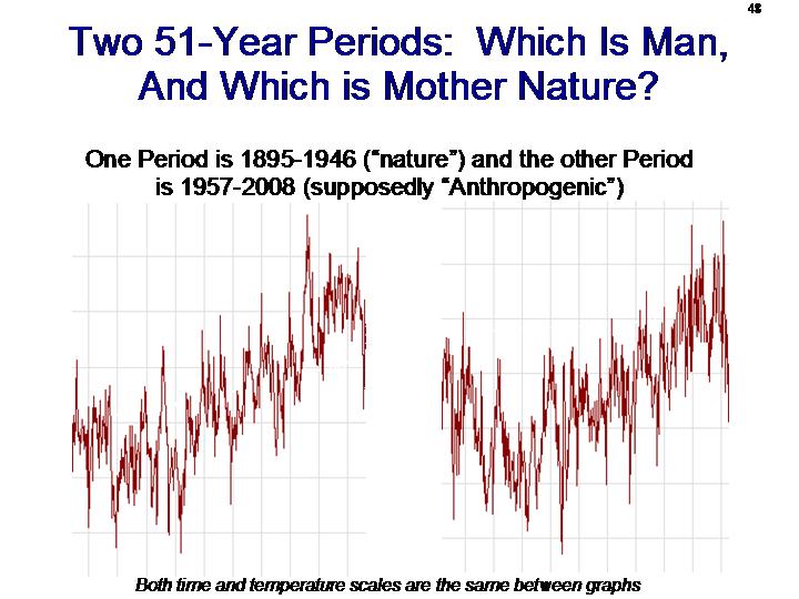
First, we have already experienced about .43 if a doubling of CO2 from pre-industrial times to today.  The same relationships and feedbacks and sensitivities that are forecast forward have to exist backwards as well.  A 15F forecast implies that we should have seen at least 4F of this increase by today.  In fact, we have seen, at most, just 1F  (and to attribute all of that to CO2, rather than, say, partially to the strong late 20th century solar cycle, is dangerous indeed).  But even assuming all of the last century’s 1F temperature increase is due to CO2, we are way, way short of the 4F we might expect.  Sure, there are issues with time delays and the possibility of some aerosol cooling to offset some of the warming, but none of these can even come close to closing a gap between 1F and 4F.  So, for a 15F temperature increase to be a correct forecast, we have to believe that nature and climate will operate fundamentally different than they have over the last 100 years.

Second, alarmists have been peddling a second analysis, called the Mann hockey stick, which is so contradictory to these assumptions of strong positive feedback that it is amazing to me no one has called them on the carpet for it.  In brief, Mann, in an effort to show that 20th century temperature increases are unprecedented and therefore more likely to be due to mankind, created an analysis quoted all over the place (particularly by Al Gore) that says that from the year 1000 to about 1850, the Earth’s temperature was incredibly, unbelievably stable.  He shows that the Earth’s temperature trend in this 800 year period never moves more than a few tenths of a degree C.  Even during the Maunder minimum, where we know the sun was unusually quiet, global temperatures were dead stable.

This is simply IMPOSSIBLE in a high-feedback environment.  There is no way a system dominated by the very high levels of positive feedback assumed in Romm’s and other forecasts could possibly be so rock-stable in the face of large changes in external forcings (such as the output of the sun during the Maunder minimum).  Every time Mann and others try to sell the hockey stick, they are putting a dagger in teh heart of high-positive-feedback driven forecasts (which is a category of forecasts that includes probably every single forecast you have seen in the media).

For a more complete explanation of these feedback issues, see my video here.

Steve McIntyre on the Hockey Stick

I meant to post this a while back, and most of my readers will have already seen this, but in case you missed it, here is Steve McIntyre’s most recent presentation on a variety of temperature reconstruction issues, in particular Mann’s various new attempts at resuscitating the hockey stick.  While sometimes his web site Climate Audit is hard for laymen and non-statisticians to follow, this presentation is pretty accessible.

The First Rule of Regression Analysis

Here is the first thing I was ever taught about regression analysis — never, ever use multi-variable regression analysis to go on a fishing expedition.  In other words, never throw in a bunch of random variables and see what turns out to have the strongest historical relationship.  Because the odds are that if you don’t understand the relationship between the variables and why you got the answer that you did, it is very likely a spurious result.

The purpose of a regression analysis is to confirm and quantify a relationship that you have a theoretical basis for believing to exist.  For example, I might think that home ownership rates might drop as interest rates rose, and vice versa, because interest rate increases effectively increase the cost of a house, and therefore should reduce the demand.  This is a perfectly valid proposition to test.  What would not be valid is to throw interest rates, population growth, regulatory levels, skirt lengths,  superbowl winners, and yogurt prices together into a regression with housing prices and see what pops up as having a correlation.   Another red flag would be, had we run our original regression between home ownership and interest rates and found the opposite result than we expected, with home ownership rising with interest rates, we need to be very very suspicious of the correlation.  If we don’t have a good theory to explain it, we should treat the result as spurious, likely the result of mutual correlation of the two variables to a third variable, or the result of time lags we have not considered correctly, etc.

Makes sense?  Well, then, what do we make of this:  Michael Mann builds temperature reconstructions from proxies.  An example is tree rings.  The theory is that warmer temperatures lead to wider tree rings, so one can correlate tree ring growth to temperature.  The same is true for a number of other proxies, such as sediment deposits.

In the particular case of the Tiljander sediments, Steve McIntyre observed that Mann had included the data upside down – meaning he had essentially reversed the sign of the proxy data.  This would be roughly equivalent to our running our interest rate – home ownership regression but plugging the changes in home ownership with the wrong sign (ie decreases shown as increases and vice versa).

You can see that the data was used upside down by comparing Mann’s own graph with the orientation of the original article, as we did last year. In the case of the Tiljander proxies, Tiljander asserted that “a definite sign could be a priori reasoned on physical grounds” – the only problem is that their sign was opposite to the one used by Mann. Mann says that multivariate regression methods don’t care about the orientation of the proxy.

The world is full of statements that are strictly true and totally wrong at the same time.  Mann’s statement in bold is such a case.  This is strictly true – the regression does not care if you get the sign right, it will still get a correlation.  But it is totally insane, because this implies that the correlation it is getting is exactly the opposite of what your physics told you to expect.  It’s like getting a positive correlation between interest rates and home ownership.  Or finding that tree rings got larger when temperatures dropped.

This is a mistake that Mann seems to make a lot — he gets buried so far down into the numbers, he forgets that they have physical meaning.  They are describing physical systems, and what they are saying in this case makes no sense.  He is essentially using a proxy that is essentially behaving exactly the opposite of what his physics tell him it should – in fact behaving exactly opposite to the whole theory of why it should be a proxy for temperature in the first place.  And this does not seem to bother him enough to toss it out.

PS-  These flawed Tiljander sediments matter.  It has been shown that the Tiljander series have an inordinate influence on Mann’s latest proxy results.  Remove them, and a couple of other flawed proxies  (and by flawed, I mean ones with manually made up data) and much of the hockey stick shape he loves so much goes away

We Eliminated Everything We Could Think Of, So It Has To Be Warming

I am still trying to get a copy of the article in Science on which this is based, but the AZ Republic writes:

Western forests that withstood wildfire, insect attacks and drought are now withering under an even greater menace.

Heat.

Rising temperatures are wiping out trees faster than the forests can replace them, killing pines, firs, hemlocks and almost every other kind of tree at almost every elevation from northern Arizona to southwestern Canada.

Writing today in the journal Science, a team of 11 researchers says global warming is almost certainly the culprit behind a sharp spike in tree deaths over the past several decades. The higher death rates, which doubled in as few as 17 years in some areas, coincide with a regional increase in temperature and appear unrelated to other outside factors.

Perhaps this question is answered somewhere in the unreported details, but my first reaction was to want to ask “Dendroclimatologists like Michael Mann reconstruct history from tree rings based on the assumption that increasing temperatures correlates linearly and positively with tree growth and therefore tree ring width.  Your study seems to indicate the correlation between tree growth and temperature is negative and probably non-linear.  Can you reconcile these claims?’    Seriously, there may be an explanation (different kinds of trees?) but after plastering the hockey stick all over the media for 10 years, no one even thinks to ask?

Normally, I just ignore the flood of such academic work  (every study nowadays has global warming in it — if these guys had just wanted to study the forest, they would have struggled for grant money, but make it about forest and global warming and boom, here’s your money).  The reasons I picked it out was because I just love the quote below — I can’t tell you how often I see this in climate science-related work:

Scientists combed more than 50 years of data that included tree counts and conditions. The sharp rise in tree mortality was apparent quickly. Researchers then eliminated possible causes for the tree deaths, such as air pollution, fire suppression or overgrowth. They concluded the most likely culprit was heat.

Again, I need to see the actual study, but this would not be the first time a climate study said “well, we investigated every cause we could think of, and none of them seemed to fit, so it must be global warming.”  It’s a weird way to conduct science, assuming Co2 and warming are the default cause for every complex natural process.  No direct causal relationship is needed with warming, all that is required is to eliminate any other possible causes.  This means that the less well we understand any complex system, the more likely we are to determine changes in the system are somehow anthropogenic.

Speaking of anthropogenic, I am fairly certain that the authors have not even considered the most likely anthropogenic cause, if the source of the forest loss is even man-made at all.  From my reading of the literature, nearby land use changes (clearing forests for agriculture, urbanization, etc) have a much greater affect on local climates and particularly moisture patterns than does a general global warming trend.  If you clear all the surrounding forest, it is likely that the piece that is left is not as healthy as it would have been in the midst of other forested land.

The article, probably because it is making an Arizona connection, makes a big deal about the role of a study forest near Flagstaff in the study.  But if the globe is warming, the area around Norther Arizona has not really been participating.  The nearest station to the forest is the USHCN station at the Grand Canyon, a pretty decent analog because it is nearby, rural, and forested as well.  Here is the plot of temperatures from that station:

grand_canyon_temp

Its hard to tell from the article, but my guess is that there is actually a hidden logic leap embedded.  Likely, their finding is that drought has stressed trees and reduced growth.  They then rely on other studies to say that this drought is due to global warming, so then they can get to the grant-tastic finding that global warming is hurting the forest.   But the “western drought caused mainly by anthropogenic warming” is not a well proven connection.  Warming likely has some contribution to it, but the west has been through wet-dry cycles for tens of thousands of years, and has been through much worse and longer droughts long before the Clampetts started pumping black gold from the ground.