Apparently a number of papers are "commemorating" today the 20th anniversary of James Hansen’s speech before Congress warning of catastrophic man-made global warming. So let’s indeed commemorate it. Here is the chart from the appendices of Hansen’s speech showing his predictions for man-made global warming:

I have helpfully added in red the actual temperature history, as measured by satellite, over the last 20 years (and scale-shifted to match the base anomaly in Hansens graph). Yes, 2008 has been far colder than 1988. We have seen no warming trend in the last 10 years, and temperatures have undershot every one of Hansen’s forecasts. He thought the world would be a degree C warmer in 20 years, and it is not. Of course, today, he says the world will warm a degree in the next 20 years — the apocalypse never goes away, it just recesses into the future.
This may explain why Hansen’s GISS surface temperature measurements are so much higher than everyone else’s, and keep getting artificially adjusted upwards: Hansen put himself way out on a limb, and now is using the resources of the GISS to try to create warming in the metrics where none exist to validate his forecasts of Apocalypse.
By the way, if you want more insight into the "science" led by James Hansen, check out this post from Steve McIntyre on his trying to independently reproduce the GISS temperature aggregation methodology.
Here are some more notes and scripts in which I’ve made considerable progress on GISS Step 2. As noted on many occasions, the code is a demented mess – you’d never know that NASA actually has software policies (e.g. here or here . I guess that Hansen and associates regard themselves as being above the law. At this point, I haven’t even begum to approach analysis of whether the code accomplishes its underlying objective. There are innumerable decoding issues – John Goetz, an experienced programmer, compared it to descending into the hell described in a Stephen King novel. I compared it to the meaningless toy in the PPM children’s song – it goes zip when it moves, bop when it stops and whirr when it’s standing still. The endless machinations with binary files may have been necessary with Commodore 64s, but are totally pointless in 2008.
Because of the hapless programming, it takes a long time and considerable patience to figure out what happens when you press any particular button. The frustrating thing is that none of the operations are particularly complicated.
Hansen, despite being paid by US Taxpayers and despite all regulations on government science, refused for years to even release this code for inspection by outsiders and to this day resists helping anyone trying to reproduce his mysterious methodologies.
Which in some ways is all irrelevent anyway, since surface temperature measurement is flawed for so many reasons (location biases, urban heat islands, historical discontinuities, incomplete coverage) that satellite temperature measurement makes far more sense, which is why I used it above. Of course, there is one person who fights hard against use of this satellite methodology. Ironically, this person fighting use of space technology is … James Hansen, of the Goddard Institute for Space Studies of NASA! In our next episode, the head of the FCC will be actively fighting for using the telegraph over radio and TV.
Robert Goddard must be spinning donuts in his grave right now.
“Great” moments, maybe (rather than “Gret” — or maybe I didn’t get the joke)? You can cut ‘n paste an extra “a” if you need one!
I enjoyed the post, but I’d think that if you did a moving avg. (on the data you supplied) over the past 20 years, you’d see small upward slope. 1988 to 1998 looks probably flat (averaged). However, it would be hard to say there wasn’t an upward trend from 1998 to about 2003. But from 2003 forward, the trend seems flat, from the data you overlayed on the chart. Is that reasonable or am I missing something?
Sedulous – I think the most interesting thing is that even if smoothed, the observed curve falls below Hansen’s “C” scenario which “drastically reduces trace gas emissions between 1990 and 2000” Sure, there might be a slight uptrend for the last 10 years depending on how you slice and smooth the data, but nothing like Hansen predicted.
Sedulous and Josh,
FOr comparison on climb, steady or fall have a look at the latest post on Watts up with that http://wattsupwiththat.wordpress.com/
We should, by now, be able to be more clever than linear regression (or even moving average) in looking for trends.
Josh,
I was just eyeballing it — I haven’t done the number crunching like Coyote has on this data. I agree with you completely that the actual data is nothing like Hansen’s!
Scott — great link, thanks for posting it.
If there’s a search function for this blog I would like to see why Coyote likes satellite data over ground measurements. I understand why he’s suspicious of ground measurements. I just don’t know how the satellite data is acquired and if its any better than the ground measurements. I would imagine that some methods for satellite measurements require a significant amount of atmospheric modeling for every measurement and that accuracy of better than a degree is pushing it. Since both sides argue over fractions of a degree… Guess I need to do some more research….
And to really get his point across, Hansen says to put oil executives on trial for spreading doubt about “global warming.”
Can somebody shoot this idiot already? Or at least throw him in jail for bogus science…
Remember this guy?
I am a lurker at Climate Audit. I have the Model E and the GISTEMP code. I am a long term computer hobbyist who has done some work porting code for statistical analysis of spectometer data collected by Analog to Digital converters. We were doing lipoprotein cholesterol analysis back in the early 80s. I’ve done darkroom work for electron microscopy. Never would Hansen have gotten a Ph D or an MD degree from the University that I attended. His thesis would have been laughed at out loud and rejected on statistical analytic grounds. And yes, his code is torture, not just a pain, it is torture and the cynic in me says that it is torture deliberately to prevent replication (which is another reason why his thesis would have been rejected).
Thanks for the Blast From The Past!!!
Nothing like bringing current issues into context.
I bet that in mid 1998.James was floating on air.Thinking that the huge warming early in the year was going to zoom like an early goddard rocket.
Now 10 years later no clear warming trend can be rationally claimed.
Now we see that James shows no humility to the fact that he is being invalidated by real temperature data.
I was reading an article about Ferenc Miskolczi from March of this year in Daily Tech
http://www.dailytech.com/Researcher+Basic+Greenhouse+Equations+Totally+Wrong/article10973.htm
Besides briefly covering his theory from his paper at
http://www.met.hu/idojaras/IDOJARAS_vol111_No1_01.pdf
it goes on to explain why Hansen is holding onto AGW theory for dear life — $$$$$$$. He can’t have any doubt thrown on his theory, lest it impact on the funding they’ve come to cherish.
As a layman, I see Miskolczi’s theory as plugging that last possible out for AGW proponents. In simple layman’s terms, it seems that the total of all greenhouse gases in the atmosphere are in stasis; add more CO2 to the mix and another GHG {H2O} is reduced. So, all things being equal, there will be no warming or cooling. Of course, all things are not equal. There is the small matter of solar variability and from that we get changes in the climate. Pity this hypothesis is not being pushed with full vigor into the face of AGW proponents and used to help put an end to all this nonsense so that we can concentrate on how to respond to real climate changes over which we will never have any power to control.
If the Oil company execs are to be put on trial…then it’s only fair that we put Al, Greenpeace, and every other climate alarmist celebrity on trial also. Once the rules of evidence apply things might get interesting. 🙂
john-
funny you should mention it…
these spanish owners and developers of beachfront property are suing greenpeace for the nagative effect their alarmist sea level predictions have had on property values.
http://www.expatica.com/es/articles/news/Estate-owners-sue-Greenpeace-for-alarming-prediction.html
Leon,
There’s a problem with Miskolczi’s paper in which he takes two unrelated expressions and equates them based on what appears to be no more than a very broad analogy regarding the Virial theorem. See the last two posts here at ClimateAudit for a more technical discussion. (And I’d be happy to expand.) The paper may have some valuable insights in it, and it is quite interesting background reading, but it doesn’t pass a sceptical review. There are plenty of good reasons for doubting AGW, but I’m afraid this isn’t one of them.
Hansen’s latest outburst has done nothing but make him look like the modern-day version of Samuel Parris.
Stevo,
Here is another look at Miskolczi:
http://landshape.org/enm/category/audits/miskolczi/
Yes, 2008 has been far colder than 1988 – are you really so stupid that you can’t even read the red line you drew yourself?
since surface temperature measurement is flawed for so many reasons … that satellite temperature measurement makes far more sense, which is why I used it above – as I’ve told you before, the surface record is in excellent agreement with the satellite record. Are you not able to understand this, are you deliberately ignoring it and pretending it isn’t true, or do you disagree?
Of course, there is one person who fights hard against use of this satellite methodology – how idiotic. In what way, exactly, is anyone ‘fighting’ against the use of satellite technology?
Oh he is back and snotty as usual.
Yawn……..
Plus the usual unsupported comments is back too.
The chart states it is ANNUAL MEAN GLOBAL TEMPERATURE CHANGE.
I see easily that 1998 has a warmer peak than the one in 2007.It has cooled since then.
You need to buy glasses.
You need to get a fucking brain, you stupid fuck. Read the post, look at the graph, and tell me if you agree that 2008 has been far colder than 1988.
Here’s a poem for you – I am also a “perfect rhyme denier” as half-rhymes are my preference. LOL
enjoy!
Global warming caused by man? Such a sick and ugly scam.
Folks who read and understand know that planet earth is very
Stained by man, it’s true, but here we
Differ knowing What is What – Fundamental – Obvious.
It’s not man, the ice cores scream, it’s just some plan
That’s slow and clean and has no ‘carbon offset’ sheen.
But still so many fools exist to parrot foolish words that miss
And so misunderstand that weather models aren’t so grand,
In fact, this science falls apart, it’s fragile numbers all distort
What has been going on and on, an icy age and then a warm,
Again and then again, as well, this cold and warm is cyclical…
Cycles are not weird or strange, they’re normal, though we rearrange
The numbers, it’s still so plain that nature rules and man just fools
Around with silly human games…
So many things cause nature pain – but carbon isn’t one of them!
Coal is evil, foul and nast – dread mercury with every blast!
It covers trees and oceans, too, paints every child a sickly blue,
But is it mentioned in all the talk? Not at all. Just greenhouse gas
The ‘see – oh – two’ will ‘seal our fate’ while ‘climate change’ expectorates
Upon our oceans, filling them, until they overflow on men
Who didn’t listen, didn’t care – HEY! Who left that ice-age there?
Bit by bit, the planet warms, each century just ups the norm,
This last century was just the same, no different than all of them,
No matter what bad science claims, it’s not man-made, we’re not to blame
For that, but hey – for other stuff? Now THERE’S some blame! You bet!
It’s rough!
Let’s do the solar! Wind is great! Bring back fish! Clean rivers, lakes!
Green power rules! Lets bring it on! But Global Warming?
No thanks.
I’m done.
.
©2008 Dave Stephens
Another warm reply from the resident troll.A real scientist would never be this ugly and also not even bother being in this blog.They are too busy doing something in their own scientific circles.
You are not a scientist at all.
“You need to get a fucking brain, you stupid fuck. Read the post, look at the graph, and tell me if you agree that 2008 has been far colder than 1988.”
Once again you are shifting.
Never did I imply in anyway that it was far colder.I simply stated: “It has cooled since then.” That is what I already said.I was also noting two high peaks as shown in the chart.2007 was a cooler year than 1998.It is so obvious.
There has been two distinct cooling periods since 1998.The 1998-2001 and mid 2007- may 2008.There has been only one distinct warming period since 1998.I hope you can spot it.It is so easy to find if you wear your glasses.
Meanwhile what is your opinion of Dr. of statistics James “censored” Hansen?
The mean temperature anomaly as measure by RSS for January to May 1988 was 0.1084. The average for 2008 so far is 0.001. The same figures for UAH are 1988: 0.1332, and 2008: -0.0204.
It is therefore certainly true to say that according the satellites January to May 2008 was notably cooler than the same five months in 1988. Whether the whole of 2008 will prove to be cooler than the whole of 1988 remains to be seen, but of course 1988 was right in the middle of the warming period that lasted from 1979 to 1997; and it is much more sensible to look at the long term trend rather than just comparing one year with another.
Rather more important is the fact that according to UAH, RSS and even the (IPCC preferred) HadCRU there has been no OLS global warming trend at all for the last 11 years, since June 1997. This has been shown at a number of interesting sites but anyone can prove it for themselves if they paste the temperature readings for the last 132 months into a spreadsheet and apply the SLOPE function.
I think Dr.Hansen has done a lot of damage to science with his alarmism and politicization of science. His unending visibility (not censorship as he claims) has had a negative effect on science in general. This trend can be seen in academia also: science with political comment. For example, on the University of CA at San Diego’s web site for their Climate Change course, http://earthguide.ucsd.edu/virtualmuseum/climatechange2/cc2syllabus.shtmleducation, you can see this editorial/political commentary creep in with ad hominem attacks on those who disagree with them. It is not a bad presentation on the whole but at one point the instructor, Wolfgang H. Berger, shows an unprofessional snarkiness at those critics who don’t buy into the computer models, thinking they are smarter than computers. He compares the climate models to the IBM Computer Chess program that beat a human, as if they are of the same scale of input — inputing chess rules vs selecting all of the factors that affect and influence climate. He should know better. At the end of the series, he comments on a Wall Street Journal editorial that argues that human progress on the whole brings much greater benefit than harm to the world. He states, “Like that of the stone age shamans assuring their people that everything is under control, the world of the writers of those editorials is an imaginary one, based on wishful thinking. Mantras and magic will do nothing to solve the problems that will come with overpopulation and the overuse of resources.” This belongs in a science course? I think not. This type of scientific pollution needs to be cleaned up so that future scientists know that policy makers depend on their data not on their political opinions.
Off topic: Can we refrain from name calling and foul language? Can we be civilized in this forum?
Isn’t is possible to delete the posts with rude profanity? Other than that this site is a good one for middle schoolers to browse to keep up on the climate debate. Can we not have moderation such that profane posters are warned and then, if they do not rein in their language, banned?
Sedulous,
There was a decent thread on WattsUpWithThat on satellite measurements. One of the issues is how UAH MSU and RSS MSU translate their measurements into temperatures, and there is a link to a site that explains the process. If you want help in finding that, let it be known; I am sure somebody could find it rather quickly.
A COMMENT IN GENERAL:
An interesting note on Hansen’s 1988 scenarios. Scenario A is business-as-usual with emissions rising @ 1.5% per year. Scenario B assumes resource constraints and environmental legislation combining to cause no increase in emissions. Scenario C was a dream. At some point in time, Hansen labeled B as the baseline scenario — the most likely scenario. In reality CO2 emissions have followed Scenario A — which of course has projections way above actual observations. Nevertheless, there could be an argument that total emissions have more closely matched Scenario B. The Montreal Protocol of 1987 led to significant Western reductions in gases which are also greenhouse gases. We cannot really check whether actual total greenhouse emissions match Scenario B or Scenario A better — Hansen used proxies and relationships for inputs (not specific numbers for various greenhouse gases) which leave most folks (including myself) quite confused.
Also, the code for Hansen’s 1988 projections can no longer be run on computers so that avenue of verification is closed.
One should give leeway for modelers to update their models based on most up-to-date information. And I certainly would give Hansen the freedom to update his models. However, there is nothing in his record which suggests to me that he has improved his models or even taken adequate steps to document his procedures.
An Inquirer – you obviously either haven’t read the paper, have misunderstood it or are deliberately misreporting it. The scenarios are not as you describe. In scenario B, emissions continued to rise, and in the real world, emissions have followed a track closest to that assumed in scenario B. They have been nowhere near the exponential rise assumed in scenario A. At some point in time, Hansen labeled B as the baseline scenario – that point in time was in 1988, in the paper.
Scientist,
In your zeal to chide An Inquirer you neglected to provide the URL and page references that could support your assertions. Knowing that it is modus operandi for all AGW advocates to back up all assertions with direct references I can only assume you were overtaken with excitement and neglected the responsibility that comes to those who presume to occupy the moral high ground.
Let me assist you.
Hansen et al, 1988, is available at http://pubs.giss.nasa.gov/docs/1988/1988_Hansen_etal.pdf
Description of the trace gas scenarios begins on page 9343. My transcription below:
“Scenario A assumes that growth rates of trace gas emissions typical of the 1970s and 1980s will continue indefinitely…”
“Scenario B has decreasing trace gas growth rates, such that the annual increase of the greenhouse climate forcing remains approximately constant at the present level.”
“Scenario C drastically reduces trace gas growth between 1990 and 2000 such that greenhouse climate forcing ceases to increase after 2000.”
I’m reading the paper again, and don’t see anywhere where the authors state that Scenario B is the baseline. You are probably confusing Jim Hansen’s testimony before Congress with the following text from the paper, “Scenario B is perhaps the most plausible of the three cases.” (Hansen et al, 1988, p. 9345)
Now as to your ability to parse English. An Inquirer states in his post above “Scenario B assumes resource constraints and environmental legislation combining to cause no increase in emissions.” Let me help you understand what “no increase in emissions” means. This means that the amount of CO2 and other trace gasses emitted each year by mankind do not increase, ie. get bigger over time. In Scenario B as described by Hansen et al, emissions do not increase. Your attempt to reinvent the meaning of emissions or increase doesn’t change the fact that An Inquirer’s description of Scenario B is consistent with the scenario described in the paper.
The actual trace gas concentrations from the three scenarios are provided online at realclimate.org . Looking at the values for CO2 for A and B from 1984 to 2007 you no doubt observed that Scenario A behaves essentially linearly at this scale. The net difference between the two scenarios is a whopping 1.6 ppm. Now compare that to the observed (where you ask? Why here of course) and the astute scientist notes that the increase in global CO2 since roughly 1998 is more consistent with the exponential senario than the linear scenario.
As to relevance, your nit with An Inquirer demonstrates a complete incapacity to understand that how closely the observed trace gas levels matched a particular scenario is menaningless if the resulting model outputs of that scenario are at odds with observed global mean temperatures. Scenario B may be the closest match in terms of the estimated trace gas forcing, but observed global mean surface temperature anomaly comes in below the projection for Scenario C.
Just an aside, Scientist, has Hansen or any other AGW scientist ever published proof that increasing the concentration of carbon dioxide in a gas sample from 0.035% to 0.045% has caused there to be an increase in the temperature of the sample upon exposure to sunlight? Something this simple would provide empirical and reproducible evidence to support his computer models and assumptions. I’ve not found any such test results listed anywhere.
Y’know, off the subject, and because it amuses me to say so, Scientist reminds me of Captain Planet. Think about Captain Planet’s theme song – “Captain Planet, he’s a hero…”
What does this say? It SAYS he’s a hero. It has to, because it’s not self-evident from his activities that he’s not just an ecoterrorist in spandex. It begs the case.
Scientist, in a similar fashion, must have realized coming into everything that it wasn’t self evident that what he/she/it was saying would be scientific. So he/she/it therefore decided to try to strengthen his/her/its case by attempting to beg the science in advance.
Earle Williams – try reading again your quote from Hansen et al: Scenario B has decreasing trace gas growth rates, and your interpretation of it: In Scenario B as described by Hansen et al, emissions do not increase. Do you really think that ‘decreasing growth rates’ means the same thing as ‘no increase’?
D.K. Wells – John Tyndall showed that this was so, in 1861.
No, Scientist, a quantitative experiment based upon the concentrations being discussed by Jim Hansen. Tyndall did experiments showing that carbon dioxide was a greenhouse gas, yes, but he did conclude that water vapor was the primary greenhouse gas with the largest effect on temperature.
http://en.wikipedia.org/wiki/John_Tyndall#Scientific_influence
No, the type experiment I’m asking about is something simple where the only variable in the experiment is the concentration of carbon dioxide. Something like two giant sealed glass containers with thermocouples to monitor the heat inside each, sitting in the middle of a giant field with a color consistent background around each. Fill each container with a gas sample made up of nitrogen, oxygen, and carbon dioxide. Leaving out water vapor and other greenhouse gases would remove them from the temperature variance equation, leaving only carbon dioxide as the variable. Have one container at a regular atmospheric concentration of carbon dioxide, 350 parts per million. Have the other at Hansen’s “tipping point” of 450 ppm. To have a good time frame, we could let this last a year.
The glass might trap some heat, but it will be similar in each. You should be able to track the heat build up in each enclosed environment with ease, and be able to have statistical proof whether there is any significant difference in the temperature of each container. If there is a significant difference, you will have proved your point, and in a relatively inexpensive manner.
Scientist,
I certainly do believe that decreasing growth rates means no increase in emissions. Apparently the concept is too difficult for you to grasp without assistance. Let me take you by the hand and explain it in smaller words. Maybe then you will begin to understand the words that you are reading but fail to comprehend.
Scenario A describes a constant growth rate of 1.5 percent. That means the amount of growth during a year is 15/1000 of the existing amount that year. The next year the amount of growth will again be 1.5% of the current amount of greenhouse trace gasses. If your starting point for a given trace gas is C, at the end of year one it will be 1.015 times C, at the end of year two it will be 1.030225 times C, year three it will be ~1.04568 * C and so on.
What you neglected to include in your quote of Hansen et al is this: such that the annual increase of the greenhouse climate forcing remains approximately constant at the present level. The trace gas level grows at a constant level. As in linearly. as in the same amount every year. Regardless of how much the value of the trace gas is in a given year the amount it increases will be same. Constant. No change.
Where you are thoroughly confused is in the understanding of the word emissions. Emissions are the amount of the greenhouse trace gas released into the atmosphere in a given year. Here I will introduce you to the word implicit. Implicit in the scenarios is the assumption that increases in the concentration of a trace gas are solely due to emissions.
Here, let me spell it out more clearly:
emissions = annual increase in trace gas concentration
If the annual increase in a trace gas concentration does not change from year to year, it is considered constant. Such a constant value, by definition, does not increase.
Careful now, we’re coming to a tricky part. If the annual annual increase in the value remains constant from year to year, and the concentration of the trace gas increases each year, then the size of the increase becomes proportionally smaller each year. Got that? maybe an example will make it clearer. If the annual increase is 2 parts per million by volume (ppmv) and the initial concentration C of the trace gas is 380 ppmv then the growth rate for that year is about 0.526 percent. After five years the concentration will be 390 ppmv. The next increase of 2 ppmv will be only around 0.513 percent. So here we have a decreasing growth rate with a constant annual emission of 2 ppmv.
This concept is pretty basic and I would expect any scientist, “scientist”, or even a Scientist to understand it. Rather than trashing other people’s understanding of science your should first make sure yours in order.
DK Wells – yes, Tyndall did experiments with CO2 as the only variable. It is beyond ridiculous to think that the physical nature of CO2 has not been investigated in this way. The effect of changing its concentration on the radiative balance of a sample of gas has not been seriously doubted for at least a century.
Earle – oh dear. How desperate to patronise you seem to be, and yet how unable to comprehend simple terminology. Scenario A = emissions increasing with a constant growth rate. Scenario B = emissions increasing with a declining growth rate. Emissions increase in both scenarios. You are obviously confused by the statement that the annual increase in forcing will remain constant in scenario B. Do you know what logarithms are?
You seem to have the paper to hand. Try reading page 9361. It is all laid out again there. Now, in future posts, try not to be such a complete dickhead.
OK, Scientist, did he do them for such small amounts as I detail? If so, could I please have a reference to the data from this work? I have searched for such results on the Internet and have not found a single reference. Doing a study where the sample represented 25% of the sample and then doubling the sample to 50% would not be the same as going from 0.035% of the sample to even doubling it to 0.070%. It is the effect with a small concentration I’m looking for, and to see if there was indeed a significant change in the overall temperature of the sample when the concentration is the same as for the standard atmospheric components.
Try reading this.
A couple of problems here, Scientist. First, no display of a mathematical relationship between CO2 concentration and temperature change observed. I won’t pull up citation material based upon the invalidation of Arrhenius’ computations as the paper itself cites that in its footnotes at the end. But my biggest problem deals with this passage from the paper:
“The assistant reported that the amount of radiation that got through the tube scarcely changed when he cut the quantity of gas back by a third. Apparently it took only a trace of the gas to “saturate” the absorption — that is, in the bands of the spectrum where CO2 blocked radiation, it did it so thoroughly that more gas could make little difference.(7*)”
That seems to say, at least to me, that once the carbon dioxide is in the system, regardless of the quantity, there was no change in the absorption saturation. So adding more did not change the absorption factor, which therefore would not change the amount of heat “trapped” by the gas.
I find it thoroughly offensive how shamelessly you’ve quoted that out of context. Your denialist agenda is now obvious. Or did you actually not read on, and find that the lab assistant had made experimental errors?
Yes, I did. And it said the errors were connected to the limits of the measuring instruments he had at his disposal. Nothing was said that the experiment was repeated then or since with more reliable instruments, showing an increase in the absorption rate. Do you have another source showing information from a repeated experiment? Or a source with a quantitative relationship between the amount of carbon dioxide (at atmospheric concentrations)and a rate of temperature increase?
Did you see this?
http://news.yahoo.com/s/afp/20080625/sc_afp/sciencegeologyoceansvolcano
Scientists find evidence of huge, violent volcanic activity under the Arctic ocean as late as 1999.
Might that melt some ice?
DK Wells – as you make no apology for quoting a result clearly stated to be in error, it is rather obvious that you are interested purely in denial, and not in science. This attitude is utterly tiresome. Read the whole of this. The whole of it. Note the point in it which says that if you want a thorough understanding of the greenhouse effect, equations and all, you won’t find it on the web. Follow the advice and get yourself a text book. Learn from it.
And do yourself a favour and in future, don’t make yourself look like an idiot by selectively quoting in the most obvious imaginable way, just to try to find backing for your preconceived and mistaken views.
dicentra: how about considering the evidence? Since 1979, Arctic sea ice coverage has shrunk by about two million square kilometres. That decline has been fairly smooth. Its rate did not change in 1999.
Now, how about a little calculation? Two million square kilometres of ice has been lost, and let’s assume for convenience that the typical ice thickness is one metre. So, two thousand cubic kilometres of ice has been lost. The density of ice is about 1g/cm³, so the mass of ice lost is 2e18 g. The latent heat of fusion of water is 334 J/g. So, the energy required to melt that much ice is 6.7e20 J. The greatest volcanic eruption in recorded history was that of Mount Tambora in 1815. The energy released in that eruption was 8.4e19 J. The eruptions on the Arctic sea floor are tiny compared with the colossal Tambora eruption, and to melt any ice at all they’d also have to heat up a column of water 4km deep. So, the amount of ice melted by Arctic sea floor activity is completely negligible.
“DK Wells – as you make no apology for quoting a result clearly stated to be in error, it is rather obvious that you are interested purely in denial, and not in science. This attitude is utterly tiresome. Read the whole of this. The whole of it. Note the point in it which says that if you want a thorough understanding of the greenhouse effect, equations and all, you won’t find it on the web. Follow the advice and get yourself a text book. Learn from it.
And do yourself a favour and in future, don’t make yourself look like an idiot by selectively quoting in the most obvious imaginable way, just to try to find backing for your preconceived and mistaken views.”
Translation:
I have run out of counterpoints to make that might be undestandable and reasonable.
Therefore I will just go to plan B and throw out a link that does not answer DK at all.Plus the usual insulting crap we have come to expect from you.
Meanwhile you simply ducked there valid questions:
“Do you have another source showing information from a repeated experiment? Or a source with a quantitative relationship between the amount of carbon dioxide (at atmospheric concentrations)and a rate of temperature increase?”
DK has been civil with you the whole time.You could have returned it in similar fashion.
I think you ran away.
“Now, how about a little calculation? Two million square kilometres of ice has been lost, and let’s assume for convenience that the typical ice thickness is one metre. So, two thousand cubic kilometres of ice has been lost. The density of ice is about 1g/cm³, so the mass of ice lost is 2e18 g. The latent heat of fusion of water is 334 J/g. So, the energy required to melt that much ice is 6.7e20 J. The greatest volcanic eruption in recorded history was that of Mount Tambora in 1815. The energy released in that eruption was 8.4e19 J. The eruptions on the Arctic sea floor are tiny compared with the colossal Tambora eruption, and to melt any ice at all they’d also have to heat up a column of water 4km deep. So, the amount of ice melted by Arctic sea floor activity is completely negligible.”
Gosh for once you made a reasonable post.
I have seen that article Dicentra posted.I did not believe that all those eruptions could warm up the water sufficiently to melt the ice.It is still very cold.
That is why I have not posted it at my forum.Not a credible attempt to explain why we have had some major artic ice melting.
Besides how do we know how long and how much the eruptions could have been going on for decades before we had the tools to monitor the ocean bottoms?
Scientist, I’m sorry that the article that you cited did not have the information I requested. But you were the one that cited it, so I am sure that you knew that quote was in there. As it is within the first eight paragraphs of the listing(as well as the information that the first global warming scientist, Arrhenius, made significant errors in his hypothesis), you should assume that it will be an article that causes immediate doubt about the global warming side of this debate.
The article also states that theoretical work on the debate stagnated for thirty years following Angstrom’s work, and never states that even a rudimentary relationship whereby one could say that x amount of carbon dioxide will cause y amount of an increase in temperature was authoritatively developed. Most of the temperature increases are based upon a doubling of carbon dioxide and estimates of the temperature increase varying from a total of 2 to 4 degrees Celsius (3.6 to 7.2 degrees F).
Nowhere in the article is there even a mention of a simple experiment such as I describe. All the listings for temperature are based upon the supposition of warming in the atmosphere. The atmosphere in toto might be a closed system, but the number of variables in it is greater than one. A definable experiment based upon the scientific method should only have one variable involved for determining a result where one can definitively state that A causes B.
Most of the article is involved with stating that the early climatologist got everything wrong. It isn’t until Callendar, Suess, Revelle, and Keeling that article even seems to be remotely supportive of any scientific contribution along this line of inquiry. Effectively, this article consigns the first hundred years of climatic atmospheric and gaseous study to the trash heap. The first truly positive note in the article doesn’t come until it cites the Princeton computer models that have been linked to Robert Hansen.
All and all, not a bad article for a history lesson. It does not address any chemical or actual real world relationships. It does reference many of the papers detailing early chemical research into the role carbon dioxide plays in the greenhouse effect. Did you notice that the article I quoted has been cited over 1900 times in scholarly papers, including a few by Hansen?
But it still fails to answer the basic question I asked you: Do you have any hard evidence to show that an increase of 100 parts per million in carbon dioxide, in a closed gas sample comprised of the major atmospheric components and carbon dioxide, produces a significant increase in temperature within that sample? A simple results chart showing increase sample by quantity X produces a temperature increase of Y will do. Said chart must define the experimental criteria that were used to achieve it so that the experiment can be reproduced if desired by a someone of average scientific training and ability, or at least understood by such a person.
Scientist,
The CO2 concentrations for the three Hansen et al scenarios are plotted here .
Note the observed CO2 as well. Compare that with your sporty quote “The scenarios are not as you describe. In scenario B, emissions continued to rise, and in the real world, emissions have followed a track closest to that assumed in scenario B. They have been nowhere near the exponential rise assumed in scenario A.”
Hehe, right. This, my friend, is known as talking out of your ass. That doesn’t fall into my version of science, but maybe it does in yours.
Just to inject a totally gratuitous note of humour in the proceedings…
http://progcontra.blogspot.com/2008/06/dr-james-hansen-speaks-out.html
I did a Google search for a quantitative analysis of CO2 to temperature and found an interesting site. They did not have an analysis, but at least they provided an explanation for why they did not. They also had some other interesting correlation studies that even suggested another possible cause for temperature variation with a higher degree of relationship than with carbon dioxid: Inflation of the British pound. They are not a peer reviewed site, and admit it from the start, but they do look at the science of the subject and are very fair handed about both sides of the argument.
http://globalwarming.chemcept.co.uk/index.htm
Seems a little hornswaggling is going on with the polar eruption/ice cap melting calculation. It appears “reasonable.” It’s certainly accurate. Problem is, it’s just not that simple.
In addition to the conductive heat transfer which the equation determines, how does adding heat (and gas?) at the ocean floor affect convective heat transfer and global currents? Has it impacted ice melt a lot, a little or not at all? I haven’t the slightest idea, but I know a snow job when I’m seeing one. Based on the available evidence this story’s nothing but good copy right now. No one knows, and given the politicization of science, I’ll be very doubtful when someone claims to know.
It’s the simple-mindedness of such calculations, foisted upon the public’s typical 4th grade scientific education that the Global WARMongers have been using to arrive at today’s hysteria.
Just some comments on the posts. As usual they are full of a majority of people with sound reasoning who reject AGW, and the few “refusers” swearing by unbelieveably ridiculous claims despite a preponderance of scientific evidence against them. Here’s a few head scratchers:
Where did anyone ever latch on to the ridiculous claim that surface measurements would be better than satellite measurements? Unless you are knowingly reading from the Hansen script, it is inconceiveable that anyone would represent themselves as knowing anything about science and make such claims. Land mass covers about 30% of the earths surface. Only 30% of land mass is within range of monitoring stations, and many of those have complicated urban temperature biases to resolve. As such surface temperature estimates are extrapolated globally from biased readings of ~10% of the planet. Steinbecks “Cannery Row” is about 100 pages. If I read you the first ten pages, how many of you could finish writing the book word for word? Not even the great Hansen could come close. Meanwhile roving satellites circle the globe collecting a temperature distribution in a matter of minutes, while geosynchronous satellites can instaneously matrix global temperatures, water vapors, infrared radiation, in the troposphere and on the surface even in places few humans have ever been. That anyone should dispute which is the more accurate measure has more to do with the fact that the satellites are making people look bad, than any scientific argument. Even if they were not clearly more accurate, they are definitely more precise and as such all predicted trends are still more trustworthy.
Also, if you cannot read a graph, please go away. The year starts with January and February, typically the coldest months in the NH. You can see that 2008 starts off with a downward trend that cannot be staved off by SH summer because of huge ice growth in Antarctica. Most hilariously as the SH headed to fall and the NH headed to summer you see a temperature plummet. This fact flies in the face of the “catastrophic” warming and ice losses at the north pole. If the North Pole is allegedly heating at an alarming rate, why does the global mean plummet as the NH heads into summer. I tutor 8th graders in pre-algebra who could pick up on this in about 1 second. Yet there are those on here screaming that the opposite is true.
Of course these are the same people who send money to Bono to cure AIDS, have starved people in developing countries because Willie Nelson told them to burn biodiesel, and have put our country’s progress 50 years behind protesting much needed power plants at the urgance of Martin Sheen. Folks, real science doesn’t get you on TV or in the newspaper. It works silently behind the scenes through strict adherence to well founded principles, to keep a balance that most idiots don’t understand and take for granted. No amount of Hero Worship will undo science. No matter who is paid what amount of money to represent what opinion, it really has no relevance on the facts or scientific reality. If you choose to keep your head buried in Algore’s ass because it provides you some feeling of comfort or security that’s fine. But no amount of time spent there, absorbing the juicy remnants of his charmed life is going to change the scientific reality that humans are not causing Global Warming if it is even happening at all. All it will get you is crap on the outside of your ears to match the crap between them.
Earle Williams – this graph shows the assumed and actual forcings. Care to tell me which scenario the observations have been closest to?
Hud – asking stupid questions without even attempting to think about them or look up answers really is a resounding hallmark of deniers. Here’s another little calculation. The arctic ocean covers an area of about 14 million square kilometres. The depth of the ocean is about a kilometre. So its volume is about 14 million cubic kilometres. The specific heat capacity of water is about 4.2 J/g/K. A cubic kilometre of water weighs about 1e15 g, so the mass of the Arctic ocean is about 1.4e22 g. So an eruption the size of Tambora would heat it up by 0.001°C, if all the energy released went into heating. That is obviously not going to affect ocean circulation or convection in any perceptible way.
Cocksman – your screed contains no science. Analogies between physical systems and literature are hardly enlightening. Noting the weather does not tell us anything about climate change. You are obviously unaware of the excellent agreement between satellite and surface temperature records. And your entirely vacuous statement that humans are not causing Global Warming if it is even happening at all demonstrates that you don’t even have crap between your ears.