Sometimes in modeling and data analysis one can get so deep in the math that one forgets there is a physical reality those numbers are supposed to represent.  This is a common theme on this site, and a good example was here.

Jeff Id, writing at Watts Up With That, brings us another example from Steig’s study on Antarctic temperature changes.  In this study, one step Steig takes is to reconstruct older, pre-satellite continental temperature  averages from station data at a few discrete stations.  To do so, he uses more recent data to create weighting factors for the individual stations.  In some sense, this is basically regression analysis, to see what combination of weighting factors times station data since 1982 seems to be fit with continental averages from the satellite.

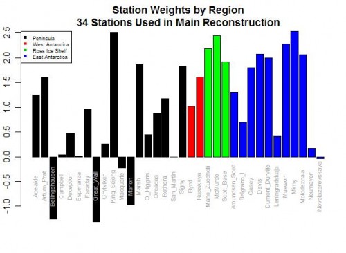
Here are the weighting factors the study came up with:

Do you see the problem?  Five stations actually have negative weights!  Basically, this means that in rolling up these stations, these five thermometers were used upside down!  Increases in these temperatures in these stations cause the reconstructed continental average to decrease, and vice versa.  Of course, this makes zero sense, and is a great example of scientists wallowing in the numbers and forgetting they are supposed to have a physical reality.  Michael Mann has been quoted as saying the multi-variable regression analysis doesn’t care as to the orientation (positive or negative) of the correlation.  This is literally true, but what he forgets is that while the math may not care, Nature does.

For those who don’t follow, let me give you an example.  Let’s say we have market prices in a number of cities for a certain product, and we want to come up with an average.  To do so, we will have to weight the various local prices based on sizes of the city or perhaps populations or whatever.  But the one thing we can almost certainly predict is that none of the individual city weights will be negative.  We won’t, for example, ever find that the average western price of a product goes up because one component of the average, say the price in Portland, goes down.  This flies in the face of our understanding of how an arithmetic average should work.

It may happen that in a certain time periods, the price in Portland goes down in the same month as the Western average went up, but the decline in price in Portland did not drive the Western average up — in fact, its decline had to have actually limited the growth of the Western average below what it would have been had Portland also increased.   Someone looking at that one month and not understanding the underlying process might draw the conclusion that prices in Portland were related to the Western average price by a negative coefficient, but that conclusion would be wrong.

The Id post goes on to list a number of other failings of the Steig study on Antarctica, as does this post.  Years ago I wrote an article arguing that while the GISS and other bodies claim they have a statistical method for eliminating individual biases of measurement stations in their global averages, it appeared to me that all they were doing was spreading the warming bias around a larger geographic area like peanut butter.  Steig’ study appears to do the same thing, spreading the warming from the Antarctic Peninsula across the whole continent, in part based on its choice to use just three PC’s, a number that is both oddly small and coincidentally exactly the choice required to get the maximum warming value from their methodology.