
The table of contents for the rest of this paper, A Layman’s Guide to Anthropogenic Global Warming (AGW) is here. Free pdf of this Climate Skepticism paper is here and print version is sold at cost here.
I mentioned earlier that there is little or no empirical evidence directly linking increasing CO2 to the current temperature changes in the Earth (at least outside of the lab), and even less, if that is possible, linking man’s contribution to CO2 levels to global warming. It is important to note that this lack of empirical data is not at all fatal to the theory. For example, there is a thriving portion of the physics community developing string theory in great detail, without any empirical evidence whatsoever that it is a correct representation of reality. Of course, it is a bit difficult to call a theory with no empirical proof “settled” and, again using the example of string theory, no one in the physics community would seriously call string theory a settled debate, despite the fact it has been raging at least twice as long as the AGW debate.
One problem is that AGW is a fairly difficult proposition to test. For example, we don’t have two Earths such that we could use one as the control and one as the experiment. Beyond laboratory tests, which have only limited usefulness in explaining the enormously complex global climate, most of the attempts to develop empirical evidence have involved trying to develop and correlate historical CO2 and temperature records. If such records could be developed, then temperatures could be tested against CO2 and other potential drivers to find correlations. While there is always a danger of finding false causation in correlations, a strong historical temperature-CO2 correlation would certainly increase our confidence in AGW theory.
Five to seven years ago, climate scientists thought they had found two such smoking guns: one in ice core data going back 650,000 years, and one in Mann’s hockey stick using temperature proxy data going back 1,000 years. In the last several years, substantial issues have arisen with both of these analyses, though this did not stop Al Gore from using both in his 2006 film.
Remember what we said early on. The basic “proof” of anthropogenic global warming theory outside the laboratory is that CO2 rises have at least a loose correlation with warming, and that scientists “can’t think of anything else” that might be causing warming other than CO2.
The long view (650,000 years)
When I first saw it years ago, I thought one of the more compelling charts from Al Gore’s PowerPoint deck, which was made into the movie An Inconvenient Truth, was the six-hundred thousand year close relationship between atmospheric CO2 levels and global temperature, as discovered in ice core analysis. Here is Al Gore with one of those great Really Big Charts.

If you are connected to the internet, you can watch this segment of Gore’s movie at YouTube. I will confess that this segment is incredibly powerful — I mean, what kind of Luddite could argue with this Really Big Chart?
Because it is hard to read in the movie, here is the data set that Mr. Gore is drawing from, taken from page 24 of the recent fourth IPCC report.

Unfortunately, things are a bit more complicated than presented by Mr. Gore and the IPCC. In fact, Gore is really, really careful how he narrates this piece. That is because, by the time this movie was made, scientists had been able to study the ice core data a bit more carefully. When they first measured the data, their time resolution was pretty course, so the two lines looked to move together. However, with better laboratory procedure, the ice core analysts began to find something funny. It turns out that for any time they looked at in the ice core record, temperatures actually increased on average 800 years before CO2 started to increase. When event B occurs after event A, it is really hard to argue that B caused A.
So what is really going on? Well, it turns out that most of the world’s CO2 is actually not in the atmosphere, it is dissolved in the oceans. When global temperatures increase, the oceans give up some of their CO2, outgassing it into the atmosphere and increasing atmospheric concentrations. Most climate scientists today (including AGW supporters) agree that some external force (the sun, changes in the Earth’s tilt and rotation, etc) caused an initial temperature increase at the beginning of the temperature spikes above, which was then followed by an increase in atmospheric CO2 as the oceans heat up.
What scientists don’t agree on is what happens next. Skeptics tend to argue that whatever caused the initial temperature increase drives the whole cycle. So, for example, if the sun caused the initial temperature increase, it also drove the rest of the increase in that cycle. Strong AGW supporters on the other hand argue that while the sun may have caused the initial temperature spike and outgassing of CO2 from the oceans, further temperature increases were caused by the increases in CO2.
The AGW supporters may or may not be right about this two-step approach. However, as you can see, the 800-year lag substantially undercuts the ice core data as empirical proof that CO2 is the main driver of global temperatures, and completely disproves the hypothesis that CO2 is the only key driver of global temperatures. We will return to this 800-year lag and these two competing explanations later when we discuss feedback loops.
The medium view (1000 years)
Until about 2000, the dominant reconstruction of the last 1000 years of global temperatures was similar to that shown in this chart from the 1990 IPCC report:

There are two particularly noticeable features on this chart. The first is what is called the “Medieval Warm Period”, peaking in the 13th century, and thought (at least 10 years ago) to be warmer than our climate today. The second is the “Little Ice Age” which ended at about the beginning of the industrial revolution. Climate scientists built this reconstruction with a series of “proxies”, including tree rings and ice core samples, which (they hope) exhibit properties that are strongly correlated with historical temperatures.
However, unlike the 650,000 year construction, scientists have another confirmatory source for this period: written history. Historical records (at least in Europe) clearly show that the Middle Ages was unusually warm, with long growing seasons and generally rich harvests (someone apparently forgot to tell Medieval farmers that they should have smaller crops in warmer weather). In Greenland, we know that Viking farmers settled in what was a much warmer period in Greenland than we have today (thus the oddly inappropriate name for the island) and were eventually driven out by falling temperatures. There are even clearer historical records for the Little Ice Age, including accounts of the Thames in London and the canals in Amsterdam freezing on an annual basis, something that happened seldom before or since.
Of course, these historical records are imperfect. For example, our written history for this period only covers a small percentage of the world’s land mass, and land only covers a small percentage of the world’s surface. Proxies, however have similar problems. For example, tree rings only can come from a few trees that cover only a small part of the Earth’s surface. After all, it is not every day you bump into a tree that is a thousand years old (and that anyone will let you cut down to look at the rings). In addition, tree ring growth can be covariant with more than just temperature (e.g. precipitation); in fact, as we continue to study tree rings, we actually find tree ring growth diverging from values we might expect given current temperatures (more on this in a bit).
Strong AGW supporters found the 1990 IPCC temperature reconstruction shown above awkward for their cause. First, it seemed to indicate that current higher temperatures were not unprecedented, and even coincided with times of relative prosperity. Further, it seems to show that global temperatures fluctuate widely and frequently, thus begging the question whether current warming is just a natural variation, an expected increase emerging from the Little Ice Age.
So along comes strong AGW proponent (and RealClimate.org founder) Michael Mann of the University of Massachusetts. Mann electrified the climate world, and really the world as a whole, with his revised temperature reconstruction, shown below, and called “the Hockey Stick.”

Gone was the Little Ice Age. Gone was the Medieval Warm Period. His new reconstruction shows a remarkably stable, slightly downward trending temperature record that leaps upward in 1900. Looking at this chart, who could but doubt that our current global climate experience was something unusual and unprecedented. It is easy to look at this chart and say – wow, that must be man-made!
In fact, the hockey stick chart was used by AGW supporters in just this way. Surely, after a period of stable temperatures, the 20th century jump is an anomaly that seems to point its finger at man (though if one stops the chart at 1950, before the period of AGW, the chart, interestingly, is still a hockey stick, though with only natural causes).
Based on this analysis, Mann famously declared that the 1990’s were the warmest decade in a millennia and that "there is a 95 to 99% certainty that 1998 was the hottest year in the last one thousand years." (By the way, Mann now denies he ever made this claim, though you can watch him say these exact words in the CBC documentary Global Warming: Doomsday Called Off). If this is not hubris enough, the USAToday published a graphic, based on Mann’s analysis and which is still online as of this writing, which purports to show the world’s temperature within .0001 degree for every year going back two thousand years!
To reconcile historical written records with this new view of climate history, AGW supporters argue that the Medieval Warm Period (MWP) was limited only to Europe and the North Atlantic (e.g. Greenland) and in fact the rest of the world may not have been warmer. Ice core analyses have in fact verified a MWP in Greenland, but show no MWP in Antarctica (though, as I will show later, Antarctica is not warming yet in the current warm period, so perhaps Antarctic ice samples are not such good evidence of global warming). AGW supporters, then, argue that our prior belief in a MWP was based on written records that are by necessity geographically narrowly focused. Of course, climate proxy records are not necessarily much better. For example, from the fourth IPCC report, page 55, here are the locations of proxies used to reconstruct temperatures in AD1000:

As seems to be usual in these reconstructions, there were a lot of arguments among scientists about the proxies Mann used, and, just as important, chose not to use. I won’t get into all that except to say that many other climate archaeologists did not and do not agree with his choice of proxies and still support the existence of a Little Ice Age and a Medieval Warm Period. There also may be systematic errors in the use of these proxies which I will get to in a minute.
But some of Mann’s worst failings were in the realm of statistical methodology. Even as a layman, I was immediately able to see a problem with the hockey stick: it shows a severe discontinuity or inflection point at the exact same point that the data source switches between two different data sets (i.e. from proxies to direct measurement). This is quite problematic. Syun-Ichi Akasofu makes the observation that when you don’t try to splice these two data sets together, and just look at one (in this case, proxies from Arctic ice core data as well as actual Arctic temperature measurements) the result is that the 20th century warming in fact appears to be part of a 250 year linear trend, a natural recovery from the little ice age (the scaling for the ice core data at top is a chemical composition variable thought to be proportional to temperature).

However, the real bombshell was dropped on Mann’s work by a couple of Canadian scientists named Stephen McIntyre and Ross McKitrick (M&M). M&M had to fight an uphill battle, because Mann resisted their third party review of his analysis at every turn, and tried to deny them access to his data and methodology, an absolutely unconscionable violation of the principles of science (particularly publicly funded science). M&M got very good at filing Freedom of Information Act Requests (or the Canadian equivalent)
Eventually, M&M found massive flaws with Mann’s statistical approach, flaws that have since been confirmed by many experts, such that there are few people today that treat Mann’s analysis seriously (At best, his supporters defend his work with a mantra roughly akin to “fake but accurate.” I’ll quote the MIT Technology Review for M&M’s key finding:
But now a shock: Canadian scientists Stephen McIntyre and Ross McKitrick have uncovered a fundamental mathematical flaw in the computer program that was used to produce the hockey stick. …
[Mann’s] improper normalization procedure tends to emphasize any data that do have the hockey stick shape, and to suppress all data that do not. To demonstrate this effect, McIntyre and McKitrick created some meaningless test data that had, on average, no trends. This method of generating random data is called Monte Carlo analysis, after the famous casino, and it is widely used in statistical analysis to test procedures. When McIntyre and McKitrick fed these random data into the Mann procedure, out popped a hockey stick shape!
A more complete description of problems with Mann hockey stick can be found at this link. Recently, a US Congressional Committee asked a group of independent statisticians led by Dr. Edward Wegman, Chair of the National Science Foundation’s Statistical Sciences Committee, to evaluate the Mann methodology. Wegman et. al. savaged the Mann methodology as well as the peer review process within the climate community. From their findings:
It is important to note the isolation of the paleoclimate community; even though they rely heavily on statistical methods they do not seem to be interacting with the statistical community. Additionally, we judge that the sharing of research materials, data and results was haphazardly and grudgingly done. In this case we judge that there was too much reliance on peer review, which was not necessarily independent. Moreover, the work has been sufficiently politicized that this community can hardly reassess their public positions without losing credibility. Overall, our committee believes that Dr. Mann’s assessments that the decade of the 1990s was the hottest decade of the millennium and that 1998 was the hottest year of the millennium cannot be supported by his analysis.
In 2007, the IPCC released its new climate report, and the hockey stick, which was the centerpiece bombshell of the 2001 report, and which was the “consensus” reconstruction of this “settled” science, can hardly be found. There is nothing wrong with errors in science; in fact, science is sometimes advanced the most when mistakes are realized. What is worrying is the unwillingness by the IPCC to acknowledge a mistake was made, and to try to learn from that mistake. Certainly the issues raised with the hockey stick are not mentioned in the most recent IPCC report, and an opportunity to be a bit introspective on methodology is missed. M&M, who were ripped to shreds by the global warming community for daring to question the hockey stick, are never explicitly vindicated in the report. The climate community slunk away rather than acknowledging error.
In response to the problems with the Mann analysis, the IPCC has worked to rebuild confidence in its original conclusion (i.e. that recent years are the hottest in a millennium) using the same approach it often does: When one line on the graph does not work, use twelve:

As you can see, most of these newer analyses actually outdo Mann by showing current warming to be even more pronounced than in the past (Mann is the green line near the top). This is not an unusual phenomenon in global warming, as new teams try to outdo each other (for fame and funding) in the AGW sales sweepstakes. Just as you can tell the newest climate models by which ones forecast the most warming, one can find the most recent historical reconstructions by which ones show the coldest past.
Where to start? Well, first, we have the same problem here that we have in Mann: Recent data from an entirely different data set (the black line) has been grafted onto the end of proxy data. Always be suspicious of inflection points in graphs that occur exactly where the data source has changed. Without the black line from an entirely different data set grafted on, the data would not form a hockey stick, or show anything particularly anomalous about the 20th century. Notice also a little trick, by the way – observe how far the “direct measurement” line has been extended. Compare this to the actual temperatures in the charts above. The authors have taken the liberty to extend the line at least 0.2 degrees past where it actually should be to make the chart look more dramatic.
There are, however, some skeptics conclusions that can be teased out of this data, and which the IPCC completely ignores. For example, as more recent studies have deepened the little ice age around 1600-1700, the concurrent temperature recovery is steeper (e.g. Hegerl 2007 and Moberg 2005) such that without the graft of the black line, these proxies make the 20th century look like part of the fairly linear temperature increase since 1700 or at least 1800.
But wait, without that black line grafted on, it looks like the proxies actually level off in the 20th century! In fact, from the proxy data alone, it looks like the 20th century is nearly flat. In fact, this effect would have been even more dramatic if lead author Briffa hadn’t taken extraordinary liberties with the data in his study. Briffa (who replaced Mann as the lead author on this section for the Fourth Report) in 2001 initially showed proxy-based temperatures falling in the last half of the 20th century until he dropped out a bunch of data points by truncating the line around 1950. Steve McIntyre has reconstructed the original Briffa analysis below without the truncation (pink line is measured temperatures, green line is Briffa’s proxy data). Oops.
![]()
Note that this ability to just drop out data that does not fit is NOT a luxury studies have in the era before the temperature record existed. By the way, if you are wondering if I am being fair to Briffa, here is his explanation for why he truncated:
In the absence of a substantiated explanation for the decline, we make the assumption that it is likely to be a response to some kind of recent anthropogenic forcing. On the basis of this assumption, the pre-twentieth century part of the reconstructions can be considered to be free from similar events and thus accurately represent past temperature variability.
Did you get that? “Likely to be a response to some kind of recent anthropogenic forcing.” Of course, he does not know what that forcing on his tree rings is and can’t prove this statement, but he throws the data out none-the-less. This is the editor and lead author for the historical section of the IPCC report, who clearly has anthropogenic effects on the brain. Later studies avoided Briffa’s problem by cherry-picking data sets to avoid the same result.
We’ll get back to this issue of the proxies diverging from measured temperatures in the moment. But let’s take a step back and ask “So should 12 studies telling the same story (at least once they are truncated and “corrected’) make us more confident in the answer?” It is at this point that it is worth making a brief mention of the concept of “systematic error.” Imagine the problem of timing a race. If one feared that any individual might make a mistake in timing the race, he could get say three people to time the race simultaneously, and average the results. Then, if in a given race, one person was a bit slow or fast on the button, his error might be averaged out with the other two for a result hopefully closer to the correct number. However, let’s say that all three are using the same type of watch and this type watch always runs slow. In this case, no amount of extra observers are going to make the answer any better – all the times will be too low. This latter type of error is called systematic error, and is an error that, due to some aspect of a shared approach or equipment or data set, multiple people studying the same problem can end up with the same error.
There are a couple of basic approaches that all of these studies share. For example, they all rely heavily on the same tree ring proxies (in fact the same fifty or sixty trees), most of which are of one species (bristlecone pine). Scientists look at a proxy, such as tree rings, and measure some dimension for each year. In this case, they look at the tree growth. They compile this growth over hundreds of years, and get a data set that looks like 1999- .016mm, 1998, .018mm etc. But how does that correlate to temperature? What they do is pick a period, something like 1960-1990, and look at the data and say “we know temperatures average X from 1980 to 1990. Since the tree rings grew Y, then we will use a scaling factor of X/Y to convert our 1000 years of tree ring data to temperatures.
I can think of about a million problems with this. First and foremost, you have to assume that temperature is the ONLY driver for the variation in tree rings. Drought, changes in the sun, changing soil composition or chemistry, and even CO2 concentration substantially affect the growth of trees, making it virtually impossible to separate out temperature from other environmental effects in the proxy.
Second, one is forced to assume that the scaling of the proxy is both linear and constant. For example, one has to assume a change from, say, 25 to 26 degrees has the same relative effect on the proxy as a change from 30 to 31 degrees. And one has to assume that this scaling is unchanged over a millennium. And if one doesn’t assume the scaling is linear, then one has the order-of-magnitude harder problem of deriving the long-term shape of the curve from only a decade or two of data. For a thousand years, one is forced to extrapolate this scaling factor from just one or two percent of the period.
But here is the problem, and a potential source for systematic error affecting all of these studies: Current proxy data is wildly undershooting prediction of temperatures over the last 10-20 years. In fact, as we learned above, the proxy data actually shows little or no 20th century warming. Scientists call this “divergence” of the proxy data. If Briffa had hadn’t artificially truncated his data at 1950, the effect would be even more dramatic. Below is a magnification of the spaghetti chart from above – remember the black line is “actual,” the other lines are the proxy studies.
|
|

In my mind, divergence is quite damning. It implies that scaling derived from 1960-1980 can’t even hold up for the next decade, much less going back 1000 years! And if proxy data today can be undershooting actual temperatures (by a wide margin) then it implies it could certainly be undershooting reality 700 years ago. And recognize that I am not saying one of these studies is undershooting – they almost ALL are undershooting, meaning they may share the same systematic error. (It could also mean that measured surface temperatures are biased high, which we will address a bit later.
The short view (100 years)
The IPCC reports that since 1900, the world’s surface has warmed about 0.6C, a figure most folks will accept (with some provisos I’ll get to in a minute about temperature measurement biases). From the NOAA Global Time Series:

This is actually about the same data in the Mann hockey stick chart — it only looks less frightening here (or more frightening in Mann) due to the miracle of scaling. Next, we can overlay CO2:

This chart is a real head-scratcher for scientists trying to prove a causal relationship between CO2 and global temperatures. By theory, temperature increases from CO2 should be immediate, though the oceans provide a big thermal sink that to this day is not fully understood. However, from 1880 to 1910, temperatures declined despite a 15ppm increase in CO2. Then, from 1910 to 1940 there was another 15ppm increase in CO2 and temperatures rose about 0.3 degrees. Then, from 1940-1979, CO2 increased by 30 ppm while temperatures declined again. Then, from 1980 to present, CO2 increased by 40 ppm and temperatures rose substantially. By grossly dividing these 125 years into these four periods, we see two long periods totaling 70 years where CO2 increases but temperature declines and two long periods totaling 55 years of both CO2 and temperature increases.
 By no means does this variation disprove a causal relation between CO2 concentrations and global temperature. However, it also can be said that this chart is by no means a slam dunk testament to such a relationship. Here is how strong AGW supporters explain this data: Strong AGW supporters will assign most, but not all, of the temperature increase before 1950 to “natural” or non-anthropogenic causes. The current IPCC report in turn assigns a high probability that much or all of the warming after 1950 is due to anthropogenic sources, i.e. man-made CO2. Which still leaves the cooling between 1940 and 1979 to explain, which we will cover shortly.
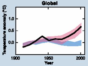
Take this chart from the fourth IPCC report (the blue band is what the IPCC thinks would have happened without anthropogenic effects, the pink band is their models’ output with man’s influence, and the black line is actual temperatures (greatly smoothed).
Scientists know that “something” caused the pre-1950 warming, and that something probably was natural, but they are not sure exactly what it was, except perhaps a recovery from the little ice age. This is of course really no answer at all, meaning that this is just something we don’t yet know. Which raises the dilemma: if whatever natural effects were driving temperatures up until 1950 cannot be explained, then how can anyone say with confidence that this mystery effect just stops after 1950, conveniently at the exact same time anthropogenic warming “takes over”? As you see here, it is assumed that without anthropogenic effects, the IPCC thinks the world would have cooled after 1950. Why? They can’t say. In fact, I will show later that this assumption is really just a necessary plug to prevent their models from overestimating historic warming. There is good evidence that the sun has been increasing its output and would have warmed the world, man or no man, after 1950.
But for now, I leave you with the question – If we don’t know what natural forcing caused the early century warming, then how can we say with confidence it stopped after 1950? (By the way, for those of you who already know about global cooling/dimming and aerosols, I will just say for now that these effects cannot be making the blue line go down because the IPCC considers these anthropogenic effects, and therefore in the pink band. For those who have no idea what I am talking about, more in a bit).
Climate scientist Syun-Ichi Akasofu of the International Arctic Research Center at University of Alaska Fairbanks makes a similar point, and highlights the early 20th century temperature rise:

Again, what drove the Arctic warming up through 1940? And what confidence do we have that this forcing magically went away and has nothing to do with recent temperature rises?
Sulfates, Aerosols, and Dimming
Strong AGW advocates are not content to say that CO2 is one factor among many driving climate change. They want to be able to say CO2 is THE factor. To do so with the historical record over the last 100 years means they need to explain why the world cooled rather than warmed from 1940-1979.
Strong AGW supporters would prefer to forget the global cooling hysteria in the 1970s. During that time, the media played up scientific concerns that the world was actually cooling, potentially re-entering an ice age, and that crop failures and starvation would ensue. (It is interesting that AGW proponents also predict agricultural disasters due to warming. I guess this means that we are, by great coincidence, currently at the exact perfect world temperature for maximizing agricultural output, since either cooling or warming would hurt production). But even if they want to forget the all-too-familiar hysteria, they still need to explain the cooling.
What AGW supporters need is some kind of climate effect that served to reduce temperatures starting in 1940 and that went away around 1980. Such an effect may actually exist.
There is a simple experiment that meteorologists have run for years in many places around the world. They take a pan of water of known volume and surface area and put it outside, and observe how long it takes for the water to evaporate. If one correctly adjusts the figures to reflect changes in temperature and humidity, the resulting evaporation rate should be related to the amount of solar irradiance reaching the pan. In running these experiments, there does seem to be a reduction of solar irradiance reaching the Earth, perhaps by as much as 4% since 1950. The leading hypothesis is that this dimming is from combustion products including sulfates and particulate matter, though at this point this is more of a hypothesis than demonstrated cause and effect. The effect is often called “global dimming.”
 The aerosol hypothesis is that sulfate aerosols and black carbon are the main cause of global dimming, as they tend to act to cool the Earth by reflecting and scattering sunlight before it reaches the ground. In addition, it is hypothesized that these aerosols as well as particulates from combustion may act to seed cloud formation in a way that makes clouds more reflective. The nations of the world are taking on sulfate and particulate production, and will likely substantially reduce this production long before CO2 production is reduced (mainly because it is possible with current technology to burn fossil fuels with greatly reduced sulfate output, but it is not possible to burn fossil fuels with greatly reduced CO2 output). If so, we might actually see an upward acceleration in temperatures if aerosols are really the cause of dimming, since their removal would allow a sort-of warming catch-up.
Sulfates do seem to be a pretty good fit with the cooling period, but a couple of things cause the fit to be well short of perfect. First, according to Stern, production of these aerosols worldwide (right) did not peak until 1990, at level almost 20% higher than they were in the late 1970’s when the global cooling phenomena ended.
One can also observe that sulfate production has not fallen that much, due to new contributions from China and India and other developing nations (interestingly, early drafts of the fourth IPCC report hypothesized that sulfate production may not have decreased at all from its peak, due to uncertainties in Asian production). Even today, sulfate levels have not fallen much below where they were in the late 1960’s, at the height of the global cooling phenomena, and higher than most of the period from 1940 to 1979 where their production is used to explain the lack of warming.
Further, because they are short-lived, these sulfate dimming effects really only can be expected to operate over in a few isolated areas around land-based industrial areas, limiting their effect on global temperatures since they effect only a quarter or so of the globe. You can see this below, where high sulfate aerosol concentrations, show in orange and red, only cover a small percentage of the globe.
 Given these areas, for the whole world to be cooled 1 degree C by aerosols and black carbon, the areas in orange and red would have to cool 15 or 20C, which absolutely no one has observed. In fact, since as you can see, most of these aerosols are in the norther hemisphere, one would expect that, if cooling were a big deal, the northern hemisphere would have cooled vs. the southern, but in fact as we will see in a minute exactly the opposite is true — the northern hemisphere is heating much faster than the south. Research has shown that dimming is three times greater in urban areas close to where the sulfates are produced (and where most university evaporation experiments are conducted) than in rural areas, and that in fact when you get out of the northern latitudes where industrial society dominates, the effect may actually reverse in the tropics.
There are, though, other potential explanations for dimming. For example, dimming may be an effect of global warming itself. As I will discuss in the section on feedback processes later, most well-regulated natural systems have feedback mechanisms that tend to keep trends in key variables from “running away.” In this case, warming may be causing cloud formation due to increased evaporation from warmer oceans.
It is also not a done deal that test evaporation from pans necessarily represents the rate of terrestrial evaporation. In fact, research has shown that pan evaporation can decrease because surrounding evaporation increases, making the pan evaporation more an effect of atmospheric water budgets and contents than irradiance.
This is a very important area for research, but as with other areas where promoters of AGW want something to be true, beware what you hear in the media about the science. The IPCC’s fourth report continues to say that scientific understanding of many of these dimming issues is “low.” Note also that global dimming does not “prove” AGW by any means, it merely makes the temperature-CO2 correlation better in the last half of the 20th century. All the other issues we have discussed remain.
The Troposphere Dilemma and Urban heat islands
While global dimming may be causing us to under-estimate the amount of global warming, other effects may be causing us to over-estimate it. One of the mysteries in climate science today has to do with different rates of warming on the Earth’s surface and in the troposphere (the first 10km or so of atmosphere above the ground). AGW theory is pretty clear – the additional heat that is absorbed by CO2 is added to the troposphere, so the troposphere should experience the most warming from greenhouse gasses. Some but not all of this warming will transfer to the surface, such that we should expect temperature increases from AGW to be larger in the troposphere than at the surface.
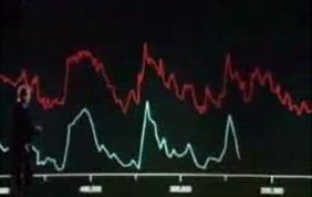
Well, it turns out that we have two ways to measure temperature in the troposphere. For decades, weather balloons have been sent aloft to take temperature readings at various heights in the atmosphere. Since the early 70’s, we have also had satellites capable of mapping temperatures in the troposphere. From Spencer and Christy, who have done the hard work stitching the satellite data into a global picture, comes this chart of satellite-measured temperatures in the troposphere. The top chart is Global, the middle is the Northern Hemisphere, the bottom is the Southern Hemisphere

You will probably note a couple of interesting things. The first is that while the Northern hemisphere has apparently warmed about a half degree over the last 20 years, the Southern hemisphere has not warmed at all, at least in the troposphere. You might assume this is because the Northern Hemisphere produces most of the man-made CO2, but scientists have found that there is very good global mixing in the atmosphere, and CO2 concentrations are about the same wherever you measure them. Part of the explanation is probably due to the fact that temperatures are more stable in the Southern hemisphere (since land heats and cools faster than ocean, and there is much more ocean in the southern half of the globe), but the surface temperature records do not show such a north-south differential. At the end of the day, nothing in AGW adequately explains this phenomenon. (As an aside, remember that AGW supporters write off the Medieval Warm Period because it was merely a local phenomena in the Northern Hemisphere not observed in the south – can’t we apply the same logic to the late 20th century based on this satellite data?)
An even more important problem is that the global temperature increases shown here in the troposphere over the last several decades have been lower than on the ground, exactly opposite of predictions by AGW theory,
In 2006, David Pratt put together a combined chart of temperature anomalies, comparing satellite measurements of the troposphere with ground temperature measurements. He found, as shown in the chart below, but as you can see for yourself visually in the satellite data, that surface warming is substantially higher over the last 25 years than warming of the troposphere. In fact, the measured anomaly by satellite (and by balloon, as we will see in a minute) is half or less than the measured anomaly at the surface.
There are a couple of possible explanations for this inconsistency. One, of course, is that there is something other than CO2-driven AGW that is at least partially driving recent global temperature increases. We will cover several such possibilities in a later chapter on alternative theories. One theory that probably does not explain this differential is global dimming. If anything, global dimming should work the other way, cooling the ground vs. the troposphere. Also, since CO2 works globally but SO2 dims locally, one would expect more cooling effect in the northern vs. the southern hemisphere, while actually the opposite is observed.

Another possible explanation, of course, is that one or the other of these data sets has a measurement problem. Take the satellite data. The measurement of global temperatures from space is a relatively new art, and the scientists who compile the data set have been through a number of iterations to their model for rolling the measurements into a reliable global temperature (Christy just released version 6). Changes over the past years have actually increased some of the satellite measurements (the difference between ground and surface used to be even greater). However, it is unlikely that the quality of satellite measurement is the entire reason for the difference for the simple reason that troposphere measurement by radiosonde weather balloons, a much older art, has reached very consistent findings (if anything, they show even less temperature increase since 1979).

A more likely explanation than troposphere measurement problems is a measurement problem in the surface data. Surface data is measured at thousands of points, with instruments of varying types managed by different authorities with varying standards. For years, temperature measurements have necessarily been located on land and usually near urban areas in the northern hemisphere. We have greatly increased this network over time, but the changing mix of reporting stations adds its own complexity.
The most serious problem with land temperature data is from urban heat islands. Cities tend to heat their environment. Black asphalt absorbs heat, concrete covers vegetation, cars and power sources produce heat. The net effect is that a city is several degrees hotter than its surroundings, an effect entirely different from AGW, and this effect tends to increase over time as the city gets larger. (Graphic courtesy of Bruce Hall)

Climate scientists sometimes (GISS – yes, NOAA — no) attempt to correct measurements in urban areas for this effect, but this can be chancy since the correction factors need to change over time, and no one really knows exactly how large the factors need to be. Some argue that the land-based temperature set is biased too high, and some of the global warming shown is in fact a result of the UHI effect.
Anthony Watts has done some great work surveying the problems with long-term temperature measurement (some of which was obtained for this paper via Steve McIntyre’s Climate Audit blog). He has been collecting pictures of California measurement sites near his home, and trying to correlate urban building around the measurement point with past temperature trends. More importantly, he has created an online database at SurfaceStations.org where these photos are being put online for all researchers to access.
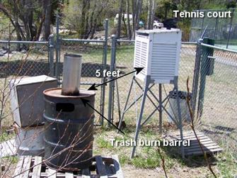

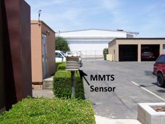
The tennis courts and nearby condos were built in 1980, just as temperature measurement here began going up. Here is another, in Marysville, CA, surrounded by asphalt and right next to where cars park with hot radiators. Air conditioners vent hot air right near the thermometer, and you can see reflective glass and a cell tower that reflect heat on the unit. Oh, and the BBQ the firemen here use 3 times a week.


So how much of this warming is from the addition of air conditioning exhaust, asphalt paving, a nearby building, and car radiators, and how much is due to CO2. No one knows. The more amazing thing is that AGW supporters haven’t even tried to answer this question for each station, and don’t even seem to care.
As of June 28, 2007, The SurfaceStations.org documentation effort received a setback when the NOAA, upon learning of this effort, removed surface station location information from their web site. The only conclusion is that the NOAA did not want the shameful condition of some of these sites to be publicized.
I have seen sites like RealClimate arguing in their myth busting segments that the global temperature models are based only on rural measurements. First, this can’t be, because most rural areas did not have measurement in the early 20th century, and many once-rural areas are now urban. Also, this would leave out huge swaths of the northern hemisphere. And while scientists do try to do this in the US and Europe (with questionable success, as evidenced by the pictures above of sites that are supposedly “rural”), it is a hopeless and impossible task in the rest of the world. There just was not any rural temperature measurement in China in 1910.
Intriguingly, Gavin Schmidt, a lead researcher at NASA’s GISS, wrote Anthony Watts that criticism of the quality of these individual temperature station measurements was irrelevant because GISS climate data does not relay on individual station data, it relies on grid cell data. Just as background, the GISS has divided the world into grid cells, like a matrix (example below).

Unless I am missing something fundamental, this is an incredibly disingenuous answer. OK, the GISS data and climate models use grid cell data, but this grid cell data is derived from ground measurement stations. So just because there is a statistical processing step between “station data” and “grid cell data” does not mean that at its core, all the climate models don’t rely on station data. All of these issues would be easier to check of course if NASA’s GISS, a publicly funded research organization, would publicly release the actual temperature data it uses and the specific details of the algorithms it uses to generate and smooth and correct grid cell data. But, like most all of climate science, they don’t. Because they don’t want people poking into it and criticizing it. Just incredible.
As a final note, for those that think something as seemingly simple as consistent temperature measurement is easy, check out this theory courtesy of Anthony Watts.
It seems that weather stations shelters known as Stevenson Screens (the white chicken coop like boxes on stilts housing thermometers outdoors) were originally painted with whitewash, which is a lime based paint, and reflective of infra-red radiation, but its no longer available, and newer paints have been used that [have] much different IR characteristics.
Why is this important? Well, paints that appear "white" and reflective in visible light have different properties in infrared. Some paints can even appear nearly "black" and absorb a LOT of infrared, and thus bias the thermometer. So the repainting of thousands of Stevenson screens worldwide with paints of uncertain infrared characteristics was another bias that has crept into the instrumental temperature records.
After running this test, Watts actually ran an experiment comparing wood that had been whitewashed vs. using modern white latex paint. The whitewashed wood was 5 degrees cooler than the modern latex painted wood.
Using Computer Models to Explain the Past
It is often argued by AGW supporters that because the historic warming is so close to what the current global warming models say historic temperatures should look like, and because the models are driven by CO2 forcings, then CO2 must be causing the historic temperature increase. We are going to spend a lot of time with models in the next chapter, but here are a few thoughts to tide us over on this issue.
The implication here is that scientists carefully crafted the models based on scientific theory and then ran the models, which nearly precisely duplicated history. Wrong. In fact, when the models were first built, scientists did exactly this. And what they got looked nothing like history.
So they tweaked and tuned, changing a constant here, adding an effect (like sulfates) there, changing assumptions about natural forcings, until the models matched history. The models match history because they were fiddled with until they matched history. The models say CO2 caused warming because they were built on the assumption that CO2 causes warming. So, unless one wants to make an incredibly circular argument, the models are useless in determining how much CO2 affects history. But we’ll get to a lot more on models in the next chapter.
The table of contents for the rest of this paper, A Layman’s Guide to Anthropogenic Global Warming (AGW) is here. Free pdf of this Climate Skepticism paper is here and print version is sold at cost here.